Using Bayesian analysis to combine and enhance MMI results

Bayesian analysis is a powerful mathematical tool that uses certain relationships from probability theory. In MMI systems, it allows a number of mental efforts from one or more users to be combined to achieve higher accuracy for difficult tasks. An example of a difficult task is predicting future events that cannot be computed from existing information, such as the numbers that will be drawn in an upcoming lottery. For simplicity I will show how to use “Bayes’ Updating” to combine multiple MMI trials to provide a single bit of information with a calculated probability of being correct.

As background, there are three types of probabilities used in Bayesian analysis. The following are their brief definitions and more commonly used notations:

  1. Joint probability is the probability of both A and B occurring.It has a number of notations.
    P(AB) = P(A and B) = P(A & B) = P(A, B) = P(A ^ B)
  2. Conditional probability is the probability A occurs given B occurs or is assumed to occur.
    P(A | B) = PB(A)
  3. Marginal probability is the total probability of observing B independent of other events. The sum of all marginal probabilities must = 1.0.
    P(B)

In addition, a number of variable names will be defined and used in the solution presented.

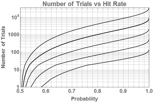
  1. Likelihood is the average probability that a measurement (a single mental effort or trial) will result in the correct answer. This is the hit rate (HR) of MMI trials. Note, the hit rate will vary both with the user and the specific type of task. Likelihood is measured and updated from real-world results. HR is always expected to be ≥ 0.5: psi missing or HR < 0.5 is not considered to be valid or useful.
  2. Prior is the presently believed probability that a specific state or answer is the correct one. The initial prior is defaulted to be 0.5, assuming there is no information to indicate otherwise.
  3. Posterior is the believed probability updated by an MMI trial (an observation or obs) that the specific state or answer is the correct one. After the posterior is calculated, its value is used as the prior for the next update.
  4. An observation, obs, is the result of an MMI trial. Obs can be either a 1 or a 0, but these symbols will typically represent an event, such as an increase or a decrease of a variable being predicted. A 1 or 0 symbol should always represent a meaning most closely associated with the symbol. A 1 will mean: up, higher, larger, stronger, faster, more, etc. A 0 will mean: down, lower, smaller, weaker, slower, less, etc. There are events or variables that have no clear or obvious association. In that case the best logical guess is used. Associate 1 with outer, even, white and hot. 0 would be associated with inner, odd, black, cold, etc. The user will learn by practice to connect the symbols with the variables. Always use the same associations.

For simplicity, the derivation of the Bayes’ updating for MMI use will not be presented here. The following algorithm and the definitions given above will allow a practical system to be implemented.

First, initialize the variables:
likelihood = hit rate determined by experience. If none is available, assume HR = 0.51;
prior = 0.5;

Calculate each posterior using a new MMI obs: Pass the three variables to the posterior function.
posterior (likelihood, prior, obs) = If (obs = 1) then,
posterior = (likelihood *prior)/((likelihood * prior) + (1 - prior)*(1 - likelihood)),
else,
posterior = ((1 - likelihood) * prior)/(prior * (1 - likelihood) + (1 - prior)*likelihood)
Return posterior.
set prior = posterior to be used as input for the next update.

Notes: the function for calculating the posterior depends on whether the obs is 1 or 0 so a conditional is used to select the proper one. It is assumed the language used calculates multiplications at a higher priority than addition so explicit parentheses are not required around multiplied variables when they are chained with additions.

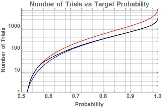
This algorithm calculates the posterior based on the assumption that the event represented by 1 is the correct one. If the posterior value returned is less than 0.5, that indicates a 0 is the true state and its probability is 1 – posterior. Generally, one wants to reach a high posterior value to have confidence it is correct and avoid false negative results. I suggest something around 0.95. This can take a large number of mental efforts, and the number is also highly variable. The number of efforts is strongly dependent on the actual HR of the user(s). When calculating a new posterior from multiple users, always use the likelihood achieved by the user who produced each obs. Entering a likelihood of 0.5 (pure chance) will not add any information nor change the posterior from the prior value.

Using incorrect likelihood values can have a number of undesirable results, though it will not prevent the algorithm from producing a result. If the likelihood is too low, a much larger number of trials can be required to reach a desired posterior value. If too high, fluctuations in posterior values will be exaggerated, causing more false negative results or reaching the threshold value too soon. If multiple users’ results are combined, misrepresenting their relative skill levels in the form of incorrect likelihoods can give too much or too little weight to their individual contributions.

Real-time user feedback is very important for best MMI results. When predicting a future event, it’s not possible to give feedback for that event since it has not yet been observed. Perhaps a trial-by-trial feedback can be given based on the size of a combined z-score or surprisal value (the ME Score for one trial). In addition, the running posterior value might be helpful, but it might also be misleading if the immediate value is in fact, incorrect, which can and will occur. Designing the best feedback will be a challenge.

One final note: in order to avoid conscious or unconscious bias, the polarity of the MMI data should be scrambled by randomly inverting blocks of data before they are combined to produce the final 1 or 0 output. The ME Trainer uses this approach for both the reveal and predict modes.

I’ve been wanting to get an understanding of Bayesian analysis for a while now so this is a good thread. Are there any application ideas you have that would be good to have this implemented in? Coding it up would be a good way for me to deepen my understanding.

In the days of PEAR research, they got effect sizes on the order of 200ppm per bit (0.0002% or p = 0.5001). MindEnabled technology raised the p value to between 0.51 and 0.70 – hundreds to thousands of times more responsive. Still not high enough or consistent enough to obtain reliable information with any single mental effort.

Bayesian analysis provides a way to make MMI applications truly useful and valuable given present-day MMI generator technology, including MED100K and some more powerful versions I have tested. Years of testing have shown there seems to be a limit on how close to 100% accuracy an MMI system can be brought by a brute-force approach of generating and processing more and more bits – up to trillions of bits in a single trial. Bayesian algorithms can take the output of multiple mental efforts and combine them to reach, at least theoretically, any desired level of accuracy.

I modeled the performance of Bayes’ updating (the simplest version) and determined how many trials or mental efforts would be required on average to reach any level of accuracy, up to 99.9%. I will provide more details later. This gives all the parameters needed to build and use MMI applications to obtain hidden or noninferable (non-computable) information.

What applications could be built using the ability to obtain even a single bit of unpredictable future information with a reasonable degree of confidence? If I played the stock market, I would like to know if a stock index was going to go up or down the next day. Just one of nearly limitless uses.

I think the first and most direct application would be a form of ME Trainer that used multiple mental efforts to produce each trial result. The ME Trainer already includes three modes: affect, reveal and predict. These are for demonstrating an affect in the MMI output to produce a bias, revealing presently existing but hidden information and predicting future information. A version of an MMI trainer would both demonstrate the functionality of Bayesian anslysis and provide a training and evaluation platform.

I should add that majority voting is also a way to combine results to obtain better accuracy. However, it is extremely limited compared to Bayesian analysis. It cannot be weighted to combine results from different users with different skill levels, nor can it take into account multiple variables drawn simultaneously from the same list of possibilities, such as 5 numbers drawn from a list of 69 (Powerball lottery).

Following is the function for calculating the resulting probability when MMI data is combined by Majority Voting, providing the average hit rate is known.

The function, pmv, returns the probability the correct symbol will be observed an absolute majority of times in n trials where the probability of observing the correct symbol in any one trial due to mental influence is HR.

pmv (HR, n) = If (HR = 1.) then return 1., else,
calculate pmv = the Sum of the terms for m = Ceiling ((n + 1)/2) to n of the equation:
Binomial (n, m) * (HR^m) * (1.- HR)^(n - m)
return pmv.

Notes: Ceiling (x) returns the smallest integer ≥ x. The up arrow, x^y, is exponentiation: x raised to the power y. Binomial (n, m) returns the binomial coefficient,
C (n, m) = n! / (m! (n - m)!).
x ! is the factorial of x. 0! = 1 by definition. Factorial grows rapidly as the argument increases, so this equation is useful for a relatively small range of n. n must be an odd integer. HR is the average hit rate for the user and task to which this equation is applied.

Example calculations:
HR = 0.51, n = 11, pmv = 0.527052274285
HR = 0.528, n = 101, pmv = 0.713837690513

How many trials are needed to reach a target probability of being correct?

The plot shows the number of trials required to reach the target posterior value. That is, the probability of being correct inferred through the Bayes’ Updating given the likelihood or hit rate provided. For this plot, the hit rate was 0.52 (effect size = 0.04). Depending on the task and the user, the actual hit rate may be higher or lower.

Trials vs Prob

The black line is the number of trials using Bayes’ Updating (BU), the blue line (bottom) is the number indicated from random walk bias amplification (RWBA) and the red line (top) is calculated using the majority voting (MV) probability equation. The number of trials for BU are bounded above by the MV and below by RWBA:
RWBABUMV

The details are somewhat complex, but note, the Bayes’ Updating method takes a constant number of trials more than the RWBA because the initial prior or starting point is assumed to be 0.5, and some trials (8 for this likelihood) are needed to get the results “up to speed.” Setting the initial prior to 0.52 removes this constant, but there is usually no information to suggest starting above or below 0.5. The number of BU trials will not exceed the MV curve, which uses a constant number of trials (an odd number starting at 1). In this portion of the curve, the BU probability equation becomes the same as the MV equation, and the numbers of trials become integers and are fixed rather than averaged.

An important confirmation from these models and simulations is that the fraction of series that reach the expected boundary first is equal to the target probability. That is, if the target probability is 0.95, the fraction of series providing a positive or true result first is 0.95 and the false negative rate is, 1 – positive rate = 0.05. The odds are 19:1 of reaching a correct result. If the target probability is set as low as 0.667, the odds of getting a correct result are only 2:1 – not very good for many practical applications. It seems likely a target of at least 0.80, giving 4:1 odds of “winning,” is a reasonable starting point.

The model also confirms the number of trials required to reach a particular target probability is very sensitive to the user’s skill level, specifically the hit rate. The number of trials is inversely proportional to the square of the effect size. That means if it takes 268 trials to reach a target probability of 80% at a hit rate of 0.52 (effect size = 0.04), it will take about 4300 trials to reach the 80% target if the hit rate is 0.505 (effect size = 0.01). On the other side, if the hit rate is 0.54, only about 67 trials will be needed. This dramatically illustrates the importance of using the very most responsive MMI hardware and processing algorithms.

The following table shows the data plotted above. Note, the numbers of trials are fixed integers up to 23 (prob = 0.576915).

Target Probability    Number of Trials         Target Probability    Number of Trials
0.52000               1.00                     0.91                  600.553
0.52998               3.00                     0.92                  648.774
0.54911               9.00                     0.93                  702.802
0.60                  33.3280                  0.94                  764.268
0.65                  66.0040                  0.95                  835.682
0.70                  113.856                  0.96                  921.203
0.75                  179.567                  0.97                  1028.56
0.80                  267.792                  0.98                  1174.92
0.81                  288.790                  0.99                  1414.50
0.82                  311.108                  0.991                 1450.00
0.83                  334.861                  0.992                 1489.45
0.84                  360.185                  0.993                 1533.89
0.85                  387.242                  0.994                 1584.86
0.86                  416.222                  0.995                 1644.74
0.87                  447.362                  0.996                 1717.50
0.88                  480.950                  0.997                 1810.57
0.89                  517.346                  0.998                 1940.64
0.90                  557.013                  0.999                 2160.89

It’s interesting to observe the number of trials needed to reach any probability or expected accuracy does not increase without bound. For p = 0.999999, N = 4323. A hundred trained users contributing about 43 trials in only several minutes, could provide one bit of information with virtual certainty. A reporter directly observing an event would not likely reach that level of accuracy.

Additional Details on using Bayes’ updating for MMI results.

Trials vs HR

This figure shows the number of trials needed to reach a target probability versus a broad range of hit rates. The bottom trace is for HR = 0.58. The other traces stepping upward reflect hit rates of 0.54, 0.52, 0.51 and 0.505. These hit rates span the range of realistically achievable levels using presently available technology.

It’s not always possible to have an exact measure of a user’s hit rate, or it may be different for the particular task at hand. Simulation is used to estimate the consequence of over- or underestimating the true hit rate (likelihood). The following three sets of parameters were examined:

  • For a nominal HR = 0.52 and a target probability of 60%. When the actual effect sizes were ±10% of the nominal value (HRs = 0.522 and 0.518), neither the number of trials nor the actual probability reached was changed in a noticeable way.
  • For a nominal HR = 0.54 (effect size = 0.08) and a target probability of 80%. When the actual effect sizes were 0.12 and 0.0533 (HRs = 0.56 and 0.5267), the numbers of trials to reach the target probability were 60 and 76 respectively. The actual probabilities reached were about 89.7 and 72.2% respectively.
  • For a nominal HR = 0.54 and a target probability of 95%. When the actual effect sizes were 0.12 and 0.0533 (HRs = 0.56 and 0.5267), the numbers of trials to reach the target probability were 155 and 273 respectively. The actual probabilities reached were about 99 and 88.3% respectively.

When the estimated hit rate is relatively close to the actual hit rate, there is little effect on the results. Underestimating the actual hit rate causes the target to be reached with fewer trials than the expected average and to arrive at a higher than the set probability target. Neither of these is detrimental to the desired outcome. Overestimating the actual hit rate causes the target probability to be reached with more than the expected average number of trials. Taking more trials than expected is not an issue by itself. When the posterior reaches 0.80, the actual probability is about 0.72 meaning the result is not as reliable as expected. With a target posterior of 0.95, the actual probability reached is about 0.883. The deficit in actual probability versus target posterior value is nearly the same in both cases (about 0.075) when the hit rate is overestimated by the same amount.

From these results it is clear that underestimating the hit rate is better than overestimating it, though it is optimal to provide a close estimate of the actual value. One way to insure against overestimating the hit rate in critical applications is to set the target probability higher than believed necessary.

The figures and equations presented here are checked and confirmed by extensive simulations. While simulations are necessary to guide and confirm proposed models, MMI effects may deviate from known mathematical models. Nevertheless, modeling and simulation can put us on track until extensive real-world testing reveals where the models are insufficient.

I want to emphasize, this example of Bayes’ updating is meant to pick between one of two possible states or correct results. These are represented by either a 1 or a 0. The equations derived for MMI Bayes’ updating give the probability that a “1” is the correct symbol. More specifically, that the event or condition associated with a 1 is the correct answer. It is just as likely that a “0”, or its associated event of condition, is the correct answer. When using the Bayes’ updating equations presented here, after each update using a new trial result, calculate threshold = Max(posterior, 1-posterior). When threshold is greater than or equal to the target probability, stop the series and take the indicated result. If posterior is the larger number, the inferred answer is the event or condition associated with 1. If 1-posterior is the greater, the inferred answer is the event or condition associated with 0.

I’m sorry to admit it. But I don’t understand that method.
Can you provide example of implementation, or formulas, how to get probability of influence from stream of data?

I have been extremely busy with issues surrounding bias amplification and increasing responsivity of MMI systems. I will provide a full write up when I have the time.

Bayesian updating is only an algorithm for processing MMI data within a complete MMI applications. It takes an MMI generator, an interface to get that data into a computer and a GUI or similar user interface for interacting with the system. Plus there is a method of training and use that provides a way of getting specific information using the whole system. Not too different than the METrainer, but that system is not set up to gain specific information.

We tried to copy your posts to GPT-4 and it generated this

Can you please write an example of algorithm code, that does amplification using BU?

I believe I provided enough detail for GPT4 to write code for the Bayesian updating algorithm. However, my experience with GPT4 is the prompt must be constructed very carefully, saying exactly and only what is needed and what is desired. It is rather good at generating code if the algorithm is clearly and exactly defined.

I also see a short sequence is used as input and the HR is set at 0.501 (ES = 0.002); too low to reach a reasonable posterior in a short sequence. I expect the output of a MED100Kx8 generator to provide a HR of 0.51 with a moderately experienced user, 10 times higher than the HR displayed in the code. I am not familiar with Python, so I can’t say if the AI got it right. I see there is a “check for convergence,” but it’s not clear to me how it is meant to work. It’s always necessary to test any code the AI provides to see if it works as expected.

GPT4 is surprisingly one of the most positive entities I have ever conversed with regarding your work, it recognizes that the science and math is sound and is happy to test these ideas, even comparing this kind of work with other major discoveries that went unrecognized at their time. I find it is best on a per function basis where you can keep all of what the code does in your mind at one time.

I have been banging my head against the wall trying to understand BU. I see you mentioned majority vote, could BU over many trials be seen as a sort of advanced majority vote? Am I reasoning about this correctly?

I assume you saw the more detailed treatment of Bayesian Updating (BU) in my paper on Advanced Processing Methods, which shows the derivation of the simple algorithm for BU in A.C.E. and MMI.

In frequentist methods, which includes MV, the test is typically aimed at calculating the probability of the null hypothesis. That is, what is the probability the trial or series of trials could be observed by chance, absent the effect (mental influence) we are interested in. There is no frequentist method I know of for calculating the probability of the alternate hypothesis, i.e., the probability that mental influence caused the observed results? In Bayesian analysis, the goal is to update the probability (posterior) indicating the presence of a particular effect with each new observation, such as more 1s or more 0s in a sampling of bits.

Briefly, frequentists calculate the probability of the results occurring in the absence of an effect, while Bayesianists calculate the probability of the presence of a particular effect. These approaches and results are fundamentally different, though both are methods of increasing accuracy in MMI results.

In the simplest measurement using a fixed number of input bits, each with a constant probability, MV is the easiest to calculate (providing advanced MV processing algorithms are not used). In this limited case, BU will give the same effect size for the same series of trials.

Ah gotcha. Yes I have been digesting the advanced data processing paper, its the first I have really dug into BU but I am starting to get it.

Given a prediction game where you guess 0s and 1s, how do you pick the value for your prior belief? I assumed it was close to .51, but does it matter if that value is for the 0s or the 1s? Or is that based on your prediction?

In BU, the likelihood is the probability the observation will be correct. It doesn’t matter if it’s for 1s or 0s. The likelihood is based on experience with the particular player, or it is defaulted to the most likely value on average. Likelihood is based on the responsivity of the MMI system, which includes the physical generator and how data is processed, but it also depends on how well the user feedback is generated and used by the player – all the parts working together.

The initial prior is the first, best guess of the correct state. If nothing is known in advance and the probabilities of any state are equal, set the initial prior to 0.5 (for two possible states). That is an “uninformative” prior, meaning there is no bias one way or the other until measurements allow posteriors to be calculated

Ah thank you, I am beginning to understand. I was confused about the initial uninformative prior values, but your explanation helped clarify things. So, regardless of the specifics of the MMI system or the user, we start with a neutral standpoint, and then as we gather more data, we adjust our beliefs. It’s all about updating our understanding based on new information. The likelihood is based on previous interactions and system responsiveness, and it adjusts as we get more feedback and data from the user. This process makes sure that the MMI system refines its predictions, making it more tailored and effective over time. I’m grateful for the clarification!

It is so fascinating that by modeling the performances of the BU you could find out how many mental efforts would be required to reach a level of accuracy. I love the idea of using a bit of future information to know if a stock would go up or down. This gives me an idea for a project of creating a crypto trading indicator based on the uniswap API, crypto and stock traders are super dedicated and focused and I could see them totally putting in the time to hone their mental efforts in order to get an edge in their trading.

What is also interesting to me is the idea of calculating a new posterior from multiple users. While experimenting with your simplified BU explanation I was able to get up to 8/10 guesses correct, but after that it was significantly more difficult for me to retain mental focus. I can see how by updating the posterior based on whichever user made the observation, you could sort of distribute the mental focus required so it wouldnt all rest on one person.

So if you had thousands of people completing trials, you’re saying not only could you use BU to gather non computable information, but you could actually predict how many trials or mental effort it would take to get an accuracy? So if one were able to create a game where a few hundred people at a time were completing trials with feedback, you could create a system to actually do stuff like predict whether a stock goes up or down? That would be such an interesting project to create.

What you describe shows you have a working understanding of Bayesian Updating in A.C.E. and MMI. There are always some more details, which we can discuss as you apply the principles of BU in real applications/games.